Today, we’ll explore what data science entails, the importance of model fitting and how we can apply it in astronomical data analysis, and the role of inference in drawing meaningful conclusions from our observations.
Inference refers to the process of comparing models to data and is a fundamental aspect of data analysis in astronomy. In the context of astronomy, model fitting enables us to extract valuable information about the physical properties of objects (like stars, galaxies, exoplanets, etc) by comparing observational data to theoretical models or mathematical functions.
This notebook will cover two of the most fundamental models with use in astronomy: lines and gaussian curves.
Linear Regression:
Linear regression just means “let’s fit a line”! It’s a statistical method used to model the relationship between a dependent variable (often denoted as ‘y’) and one or more independent variables (often denoted as ‘x’). It assumes that the relationship between the variables can be described by a linear equation, such as a straight line in the case of simple linear regression. Like an inference task, the goal of linear regression is to find the best-fitting line that minimizes the differences between the observed values and the values predicted by the model.
For the simpliest case of a straight line, aka a first order polynomial, we can describe our model using two parameters: slope and intercept.
How can we implement this in python?
np.polyfit is a function in NumPy used for polynomial regression, which fits a polynomial curve to a set of data points. In the context of linear regression, np.polyfit fits a polynomial of degree 1 (a straight line) to the given data points by minimizing the sum of squared errors between the observed and predicted values. This function returns the coefficients of the polynomial that best fits the data, allowing us to determine the slope and intercept of the regression line.
import numpy as np
import matplotlib.pyplot as plt

# Generate fake data for demonstration
x = np.array([1, 2, 3, 4, 5])
y = np.array([2.1, 3.9, 5.8, 8.2, 10.1])
# Fit a straight line (polynomial of degree 1) to the data
coefficients = np.polyfit(x, y, deg=1)
coefficientsarray([ 2.03, -0.07])# Extract the slope (m) and intercept (b) from the coefficients
slope, intercept = coefficients
# note: you can do this more efficiently by just writing: slope, intercept = np.polyfit(x, y, deg=1),
# but I wanted to print coefficients to show the actual output of polyfit
# Print the equation of the fitted line
print(f"Fitted line equation: y = {slope:.2f}x + {intercept:.2f}")Fitted line equation: y = 2.03x + -0.07
So we have managed to fit a line to our data! Horray! Now let’s plot both the data and model:
# Generate points along the fitted line for plotting
x_fit = np.linspace(min(x), max(x), 100)
y_fit = slope * x_fit + intercept

# Plot the data points and the fitted line
plt.figure(figsize=(8, 6))
plt.scatter(x, y, color="blue", label="Data")
plt.plot(x_fit, y_fit, color="red", label="Fitted Line")
plt.xlabel("x", fontsize=14)
plt.ylabel("y", fontsize=14)
plt.legend()
plt.show()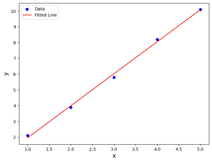
A practical astronomy application: The M-sigma Relation
The M-sigma relation, also known as the black hole mass-velocity dispersion relation, is an empirical correlation observed between the mass of supermassive black holes () at the centers of galaxies and the velocity dispersion (σ) of stars in the bulges of those galaxies. This relationship suggests that there is a tight connection between the properties of galaxies and the central black holes they host. Specifically, galaxies with larger velocity dispersions tend to harbor more massive black holes at their centers.
The M-sigma relation has profound implications for our understanding of galaxy formation and evolution, as well as the co-evolution of galaxies and their central black holes. It provides valuable insights into the mechanisms governing the growth and regulation of supermassive black holes, the role of feedback processes in galaxy evolution, and the relationship between the properties of galactic bulges and their central black holes.
What about fitting arbitrary functions?
Everything we’ve done so far pertains to fitting polynomials to data, but what if you want to fit a differnt type of function (like a Gaussian distribution)? We will go into this on Wednesday!