Functions (and HII regions in M33)

In this week’s lab, we’ll see how to construct and use Python functions in practice, using a narrowband image of the galaxy M33 as our dataset.

Our ultimate goal will be to nicely plot and crop our image to make scientific measurements of the physical size of certain features in the galaxy.

We’ll also see at the end why writing functions was a useful way to organize and carry out this analysis. We’ll start focusing just on the image. In Part II, there is a scientific overview regarding HII regions and why we are interested in them.

# Some libraries we'll need throughout
from astropy.io import fits 
from astropy.wcs import WCS 
import numpy as np 
import matplotlib.pyplot as plt

Part 0: Warm up¶

Before we dive into new things, let’s re-familiarize ourselves with how to write some simple functions.

Part 1: Loading and viewing astronomical images¶

Astronomical images (those taken at a telescope like Keck Observatory, or in space, like HST or JWST) are, at their core, a 2D array of values. In general, we take images in one band (color) at a time, and if we want color images like those you can take with a camera, we have to later combine those images.

The vast majority of astronomical images that have been, and continue to be, taken are stored in a special file format called FITS. Fits stands for Flexible Image Transport System. It’s a binary format which requires specialized programs to open. One is SAOImage DS9, a GUI based tool I recommend having if you will be working with astronomical images.

In Python, we can use the astropy.io.fits module to load the header (a dictionary of information about the file) and data (images) from a FITS file.

Within a FITS file, information is stored in what are called extensions. These are like separate buckets/folders, and thus allow one to store multiple images, or an image + table, or multiple tables, within 1 file. But usually, we have a simple file with 1 image in the 0th extension, and its header.

When we load a FITS file, we usually also want to know something about the coordinates (on the sky, so RA and DEC) of the things in our image. To do this, we need to know the WCS (world coordinate system) coordinates of the image. The information needed to make one of these is in the image header, and there is an astropy function to convert a header to a wcs object.

The code below will load the M33 image we’ve provided into Python, setting the 2D array im as the image, and the wcs object via the astropy routine.

from astropy.io import fits 
from astropy.wcs import WCS 

with fits.open('./M33_halpha.fits') as hdu:
    im = hdu[0].data 
    wcs = WCS(hdu[0].header)

We can, if we wish, encapsulate this operation into a function. It’s short enough that it’s not overly onerous to write out each time. But we can make these three lines into one, which might make our code easier to read when loading many different fits files throughout a script.

Exercise 2.2

This is already a few lines of code, and we often need to plot astronomical images. Let’s now make a function that can streamline some of these lines of code above for us.

First define a function implot. The first argument should be a variable path_or_pixels. We’re going to allow users to either provide a file name to a fits file directly, or provide an image array (as we did above). To handle this, write some logic using the isinstance() python function to check whether the input is an array or a string, and if it is a string, use the load_fits function we wrote in Exercise 1 to load the image. (Otherwise, we’ll just set our image to be the path_or_pixels input, assuming it is an array. You could use isinstance() again to check if it is a numpy array and raise an exception if not, optionally.)

Include as arguments the following:

percentiles (list) (which will let users scale vmin and vmax, set to a default of [1,99.5].
figsize (tuple): an optional argument with a default set to something like (8,8).
cmap (str): argument with a default of 'gray_r', passed along the imshow command, giving us control over the plotting color mapping.

Your function should return the fig and ax objects it created.

Hint: isinstance()

If you haven’t used isinstance() yet, here’s a primer.

When we want to check the type of a variable, we can use type(var_name) to see its typename. When we want to check or ensure that a variable’s type matches some desired type, we can use isinstance(variable,type) to return True or False. For example, isinstance('test',str) would return true, because the input 'test' is a string. The names for the built-in types are str,bool,list,dict,tuple,float,int, etc. For a numpy array, its “type” is np.ndarray.

Hint

We haven’t covered how to type-hint multiple allowed types yet. Here’s a preview hint if you want to include it, but you don’t have to:

from typing import Union 
def func(arg: Union[np.ndarray,list]):
    ...

Exercise 2.4

Now we want to incorporate the wcs into the mix.

Currently, a wcs will be accessible if the user provides the path to a file that has one. Now, add an optional argument to your function wcs with a default of None. Add logic so that if the wcs is not None (either from loading an image, or after the function input), we add the following to our subplots command:

fig, ax = plt.subplots(figsize=figsize,subplot_kw={'projection':wcs})

What this does is turn our regular axis into a WCSAxis, which can handle plotting astronomical units along the axes of our image.

Try your function again, but this time add the wcs we created in the previous exercise. How do your plot axes change?

Extra Feature (optional)

At the moment, the user chooses whether to provide a wcs for the pixels case, but we force a wcs plotting if a path to a fits file that contains a wcs is provided. This should be the default case, but it might be nice to give the option to turn that off. The easiest way to accomplish this is to add an ignore_wcs optional argument to your function which has a default of False. Thus, given an image file path, we can plot using coordinates by default, or the raw pixels by ignoring any wcs present. This works too if we provide a wcs but want to easily toggle it on and off.

There are now 13 lines of logic in our function, and hopefully it is becoming clear why making such a function is so useful --- we can now very quickly and easily load and plot any fits file, or any array we have on hand, with wcs on or off, with limits setting, all in one line.

Part II: The Size of HII Regions¶

The Science

For the rest of the assignment, we will be investigating the physical size of HII regions in nearby galaxy M33. Not sure what that means? Here’s a quick primer.

Stars form of many different masses (from much smaller than the sun to much larger), with many more low mass stars forming than massive stars $^*$ . While very few high mass (e.g., 3-10+ $M_{\odot}$ ) stars form at a time in a galaxy, they have an outsized effect, dominating the light of the low mass stars (though they live much shorter lives). They are also the only stars (dubbed O-type) who put out significant light in the ultraviolet part of the spectrum. We know that our own sun does emit some light in the UV (that’s the more high energy, dangerous light that can give us cancer, hence sunscreen), but these stars pump out most of their light in the UV.

UV light has enough energy to ionize the atoms in gas (especially hydrogen gas), which means to knock the bound electron out of the atom and leave behind a proton and an electron. In some equilibrium, these electrons recombine with protons, and the electrons cascade through several energy levels as they fall toward the ground (most bound) state. For each gap they drop, the atom emits a photon with an equivalent energy to the difference between the levels traversed.

This process of recombination produces light at specific wavelengths, so when you look at planetary nebulae, star forming regions, or supernova remnanta (see below), the colors are representitive of the different elements and energy levels being traversed.

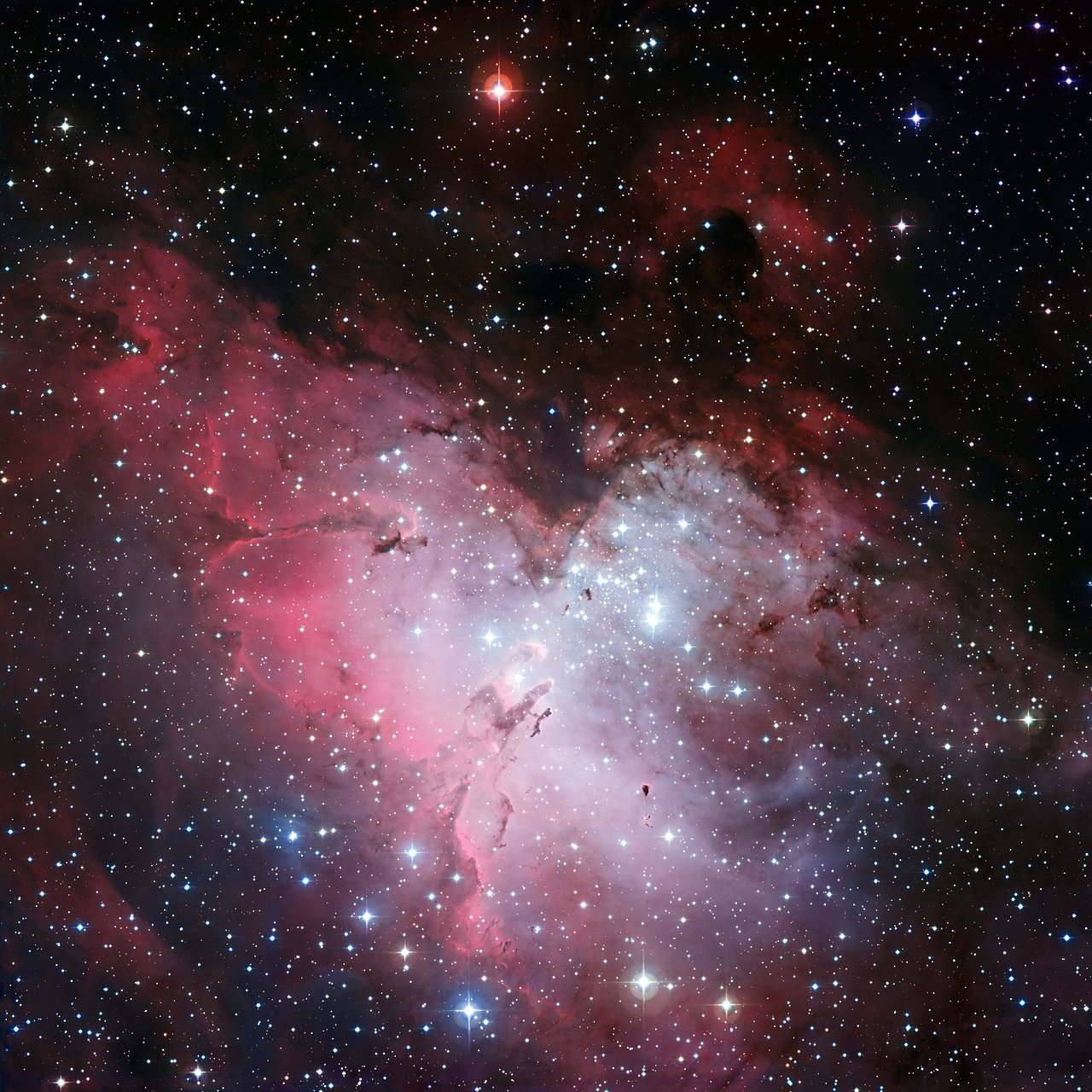eagle nebula The Eagle Nebule, where we can see the hollow region being blown out by young stars (with the famous pillars of creation remaining, soon to be whittled down. Credit: ESO

Bright, young stars actually put out enough radiation to “blow out” and push on the gas remaining from the clouds from which they formed. This carves our roughly spherical regions known as Strömgen spheres, the inner boundary of which is usually lit up in this ionized emission. The size of the sphere blown out depends on the total amount of flux coming from the bright stars, which in turn depends on how many of them there are.

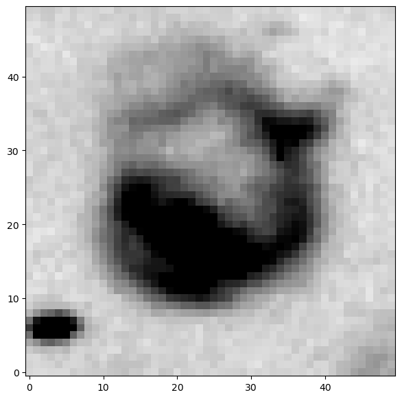
In our image of M33, we can see lots of these roughly spherical regions being highlighted by the narrow, Hα filter being used to observe the galaxy. By measuring their size in pixels and using our knowledge of the distance to M33, we can perform some simple trigonometry to determine their actual physical sizes. As a bonus, we can then roughly estimate the number of O-type stars responsible for the visible HII region. (note that Starforming region and HII region are roughly synonymous; HII is the chemical name for ionized hydrogen).

*

Stars that form together out of one more massive cloud have masses drawn from what is called an initial mass function, or IMF, which is roughly exponential.

Exercise 3.1

While we can see by eye lots of small HII regions scattered around M33 in our image, to do a more careful analysis of the sizes we will need a way to crop our images to just focus on one HII region at a time.

There are fundamentally two ways to carry out this crop. We can work in units of image pixels, and use array indexing and slicing to select subarrays containing out HII regions. Or, we could use our wcs objects to pick central coordinates on the sky and a size (in sky angular units) to crop in on, and use an astropy tool to do the crop.

In this exercise, we will work with the pixels, as it will be good practice for our array indexing and slicing.

Our first step is actually determining the pixel coordinates of a given HII region. While there are more complex methods we could write, it is not so hard to do this by eye. That said, a simple crosshairs function would help us know that our chosen coordinates land right on an HII region.

Write a function crosshairs which takes in crosshairs(ax,x,y). It should then use ax.axvline(x) and similarly ax.axhline(y) for y to plot a crosshairs over our image at some coordinates. Return ax when done.
Run you function for position (995,1445). Are you right on an HII region?

# Here is an an example of ~what you should be seeing

(<Figure size 700x700 with 1 Axes>, <Axes: >)

Exercise 3.3

You should hopefully now have a nice, circular feature filling most of your plotted image. This is our HII region!

In order to estimate its radius in pixels, we’d like to place a circle down that lines up with the ridge of emission defining the circle (and adjust our center as needed, as our by-eye estimate from the full image was likely not perfect.

Recall that we can compute the x and y values of a circle with position $(x_0,y_0)$ and radius $R$ via $x(\theta) = x_0 + R\cos(\theta)$ and $y(\theta) = y_0 + R\sin(\theta)$ . Write a function add_circle(ax,x,y,r) which takes in our image ax, creates an array of theta values from 0 to $2\pi$ (Hint: np.linspace() is good for this), computes the arrays for the x and y positions of the circle based on its center and radius, plots them using ax.plot(x,y) over the image, and returns the ax.
Use your function to determine the new center and radius $R$ of this HII region.

Exercise 3.4

Now that we have a measurement of $R_{HII}$ in pixels, we need to begin converting this to a physical scale. We can do this because we know the pixel scale of our detector, that is, how many angular degrees (here we’ll use the arcsecond) on sky does one pixel subtend. For example, if we have a pixel scale of 2.2, that means each pixel subtends 2.2 arcseconds on sky (roughly 0.0006 degrees).

We can then make a triangle --- the long edge is the distance in physical units to M33. The short edge is the length we want, the physical radius of the HII region, and θ is our measured angular radius, obtained by multiplying the radius in pixels by the pixel scale.

To perform the actual trigonometric step, we need to compute $D\tan(\theta)$ .

Write a function compute_size(distance,s_pix,pixel_scale). Using the pixel scale, it should convert the size s_pix to arcseconds, then onward to degrees (there are 3600 arcseconds in a degree), then onward to radians for the trig function (np.deg2rad() may be useful here). Then, using that, compute the size using the formula above and return it. The size output will have units equal to the length units that were assumed for $D$ .
M33 has a distance of 0.869 Mpc (Megaparsec). Using your function, compute the radius of the HII region in parsec by converting the M33 distance to pc, then using your compute size function. Assume a pixel scale of 2.2. How big is this HII region?

Exercise 3.6

Now that we know the physical size of the HII region (not a trivial feat!) we can actually go further. In a back-of-the-envelope sense, the radius of the full HII region can be approximated as that of a Strömgren sphere around a “single” high energy star.

The formula for this radius is

r_S = \left(\frac{3N^*}{4\pi\alpha n^2}\right)^\frac{1}{3}

(1)

where $N^*$ is the ionizing photon rate from the OB star (typically $\sim 10^{49}$ photon s^-1), $\alpha \sim 3\times10^{-13}$ cm³ s^-1 is the recombination coefficient, and $n\sim 10$ cm^-3 is the number density.

We know $r_S$ . Solve this equation instead for $N^*$ , writing a function that returns the value of

\left(\frac{N^*}{10^{49}}\right)

(2)

Having done so, you now have a function that given a radius and assumptions about particle density and recombination coefficient returns the “number” of OB stars driving the HII region! (Technically, we have an answer that is units of the typical OB star’s photon flux, so the actual number of stars could be lower if each is more massive and brighter and vice versa --- but this gives both the actual driving flux and an approximate order-of-magnitude estimate for the number of stars.

Play with your function a bit, putting in values from 10 pc to 500 pc for the size, and see how the ionizing flux changes!

Exercise 3.7: Putting it all together

Throughout the course of this lab, you have written several shorter (and longer) functions. For our implot function, it is hopefully clear why having that function around is handy --- to set everything we included every time we wanted to quickly view some fits file or local array would be onerous; this function now makes it very easy to get a useful result in a simple one line call, with plenty of room to specify options if we desire.

On the other hand, something we covered in lecture was that functions are most useful for reusable bits of code. Thus far, though, we only measured one HII region. In theory, all of the computations we did along the way could have been done directly in our script or notebook and it would not have been that disorganized of a file.

Let’s now demonstrate why writing functions was useful, even for the small steps.

Using the original image, pick four more HII regions in the image of M33, and determine their physical sizes and number of OB stars.

Tasked with this, hopefully you will be able to re-use your defined functions to make locating and measuring the size of each much easier! Create section headings in your solution with each one. While the solution won’t be fully automatic, since we still have some by-eye assesment happening, the final code block for doing this whole measurement will only be a few lines long, calling our pre-made functions. As we move further into the semester, we will learn how to automate, e.g., finding the locations of features of interest and measuring the size of those features.